How to Calculate Orbital Decay Rate: The Step-by-Step Satellite Guide

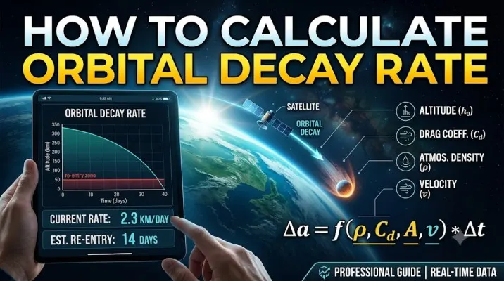
Every satellite in low Earth orbit faces the same inevitable fate. Drag from the atmosphere slowly pulls them down. Understanding how to calculate orbital decay rate matters for mission planning, collision avoidance, and predicting when a satellite will re-enter the atmosphere.

I have worked with orbital decay calculations for university satellite missions. The process looks intimidating at first. But once you break it down step by step, you will see it is manageable with the right tools and approach.

If you are searching for an orbital decay calculator, you need to understand what you are calculating and why it matters. This guide will walk you through the entire process. We will cover the physics, the math, and the practical tools you can use right now.

What Actually Causes Orbital Decay?

Atmospheric drag is the main culprit. Even at altitudes of 400-500 kilometers, there is enough atmosphere to slow a satellite down over time. The higher the satellite flies, the slower the decay. But nothing in low Earth orbit stays up forever.

Read Also: The Passive Safety Blueprint: Why Thorium Molten Salt Reactors Defy Nuclear Meltdowns?

The physics is straightforward. The satellite collides with air molecules. This transfers energy away from the orbit. The satellite loses speed and altitude. The lower it gets, the denser the atmosphere becomes. This creates a feedback loop that accelerates the decay process.

For example, a satellite at 400 kilometers might stay up for several years. At 550 kilometers, you are looking at decades before re-entry . But solar activity changes everything. When the sun is active, the atmosphere expands and causes faster decay.

The Basic Math Behind Orbital Decay Calculations

You do not need to be a rocket scientist to understand this. The orbital decay rate equation looks like this:

drdt=−64G3(m1m2)(m1+m2)5c5r3dtdr​=−5c5r364G3(m1​m2​)(m1​+m2​)​

This equation calculates how fast the orbital radius decreases over time . Here is what each symbol means:

• G is the gravitational constant (6.674 × 10⁻¹¹ m³ kg⁻¹ s⁻²)

• c is the speed of light (2.997 × 10⁸ m/s)

• m₁ and m₂ are the masses of the two bodies

• r is the orbital radius

When you plug in the numbers for two solar-mass objects at 1 million kilometers apart, you get a decay rate of about -78 centimeters per year . This is for gravitational wave emission, not atmospheric drag. But it shows you how the math works.

For satellites in low Earth orbit, atmospheric drag is the dominant force. The equation changes to account for air density and the satellite's physical characteristics.

The Practical Step-by-Step Process

1: Gather Your Satellite Data

You need specific information about your satellite:

You Must Also Like: Quantum Scrambling Reversal: Latest Breakthroughs Explained

• Semi-major axis (a) in kilometers

• Eccentricity (e) of the orbit

• Cross-sectional area (A) in square meters

• Drag coefficient (Cd) - typically around 2.2 for most satellites

• Mass (m0) in kilograms

These parameters determine how much drag the satellite experiences. A larger area means more drag. A heavier satellite resists deceleration better.

2: Get Solar Activity Data

Solar activity directly affects atmospheric density. You need two key numbers:

• F10.7 solar radio flux

• Ap geomagnetic index

These values change daily. You can find them from space weather forecasting websites. For accurate orbital decay calculations, use real-time data .

3: Choose Your Calculation Method

There are three main approaches to calculating orbital decay:

The Simple Approach

For quick estimates, use the "decay rate equals drag deceleration multiplied by Keplerian period divided by Pi" formula . This works surprisingly well for rough estimates. The math is simple enough that you can do it by hand.

The Numerical Integration Approach

For high accuracy, use numerical integration. This means calculating the drag at many points along the orbit and summing them up. The DSST (Draper Semi-analytical Satellite Theory) method is a popular choice . Other methods include the energy method and Gaussian variation method.

The Software Approach

Professional tools do all the heavy lifting for you. The Satellite Lifetime Tool in Systems Tool Kit (STK) provides accurate decay time estimates . For higher fidelity, combine it with the High-precision Orbit Propagator (HPOP). Start with the Lifetime Tool estimate, then use HPOP for precise re-entry timing.

4: Run Your Calculation

If you are using MATLAB, there is a function available that computes orbital decay for objects between 180 and 500 kilometers altitude . The function syntax is:

text

[P,t] = computeOrbitalDecay(a,e,A,Cd,m0,F107,Ap)

The output gives you the orbital period vector (P) and the propagation time (t). This is a practical orbital decay calculator you can use immediately.

Tools You Can Actually Use

NASA Debris Assessment Software (DAS)

This is the gold standard. It is used by Starlink to validate their deorbit claims . The software is available to US citizens through NASA, with a two-week approval process. It includes two utilities for deorbit analysis: Orbit Lifetime/Dwell Time and Apogee/Perigee Altitude History.

ESA's DRAMA Tool

For users outside the US, ESA offers DRAMA (Debris Risk Assessment and Mitigation Analysis) . It is available free to industry, researchers, and space organisations within ESA Member States. This is what university missions use to show compliance with space debris mitigation requirements.

Decay Analyzer Python Toolkit

There is an open-source Python toolbox available for satellite orbit decay analysis . It supports multiple analysis methods including DSST, energy method, and Savitzky-Golay filtering. This is a good option if you want to write custom code.

The Simple Web Calculator

For quick estimates, there is a simple online tool at lizard-tail.com . The downside is that it does not account for time-varying solar flux. So treat its results as rough estimates only.

Common Mistakes to Avoid

Ignoring Solar Activity

Solar flux changes atmospheric density significantly. Ignoring it can make your decay predictions completely wrong. Always use current solar data.

Using the Wrong Area Value

The cross-sectional area in the direction of drag is what matters. Assuming full solar panel area gives you artificially low decay numbers . For dead satellites, you need to know what orientation they settle into.

Assuming Constant Drag

Drag changes as the satellite descends. The atmosphere gets denser. The satellite orientation might change. Your calculation needs to account for this.

Not Validating Your Results

Always compare your results against known values. If you calculate a decay time that seems too long or too short, check your inputs.

When Simpler Is Better?

For most practical purposes, you do not need the most complex model. The ORBITM approach shows that you can calculate decay rate without full orbit propagation . The key insight is that you only need the radial distance of the spacecraft. This simplifies everything.

The closed-form solution works because the decay rate is small within a single orbital period. For a low Earth orbit at 95 minutes, you can use larger time steps without losing much accuracy. This is why some simple calculators produce useful results despite their limitations.

When You Need High Precision

If you are planning a mission that needs to hit a specific re-entry window, simple estimates are not enough. You need precision propagation. This means integrating the equations of motion with high-fidelity force models.

High-precision propagation requires accounting for:

• Non-spherical Earth gravity

• Atmospheric drag with high-quality density models

• Solar radiation pressure

• Third-body attractions from the Moon and Sun

• Earth eclipsing effects

The development of precision propagators is complex. Commercial software exists but is often packaged as closed systems. This is why many organisations develop their own tools. The results from high-end commercial software and SGP4 often have to be taken at face value .

The Final Thoughts on Orbital Decay Calculators

There is no single best orbital decay calculator. Each tool has its strengths and weaknesses.

The NASA DAS software is the most authoritative option for US users. ESA's DRAMA is the best choice for European users. For quick estimates, use a simple web calculator. For precision work, develop your own propagator or invest in professional software.

Start simple. Get a rough estimate first. Then refine your inputs and method. Validating results against known decay rates will help you choose the right tool for your specific needs.